[ planet-factor ]
John Benediktsson: Peace For All
I am perhaps susceptible to nerd-sniping and it often leads me down interesting rabbit holes. Today was one of those days. I bumped into a fun article about some obfuscated bash code on a T-shirt for sale:
The obfuscated code in question is actually an easter egg, it’s being supplied via Uniqlo stores on an excellent t-shirt designed by Akamai in support of their Peace for All campaign.
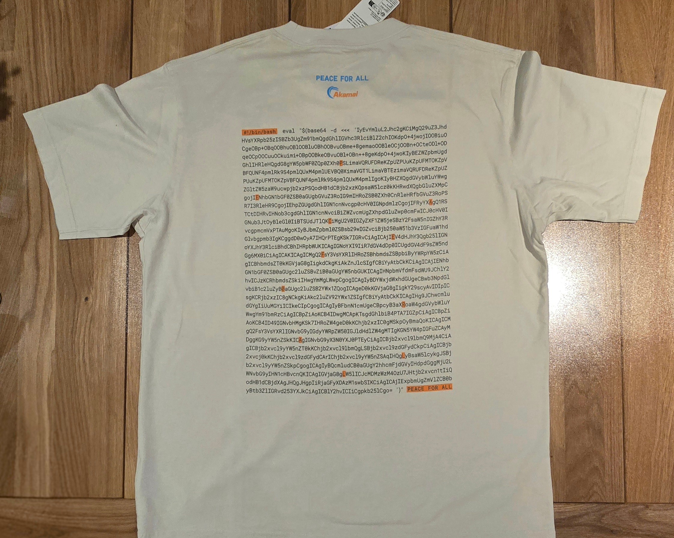
While reading about the author’s use of
OCR to
convert the printed text into a string that they could compute base64 --decode on to see the resulting program, I had major nostalgia for
carefully typing programs from computer
magazines so they could be
run locally – the only option for us kids at the time.
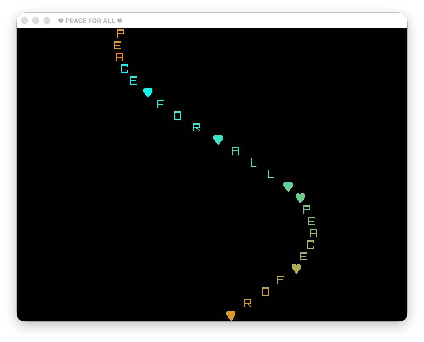
Raylib can be a great tool for doing colorful animations and is pretty well supported by Factor. I thought it would be fun to show how to write a similar program using it!
First, we define some constants for our message (infinitely looping using a circular sequence), font sizes, text colors, and then a computed number of visible text rows:
CONSTANT: message $[ "♥PEACE♥FOR♥ALL" <circular> ]

CONSTANT: width 800
CONSTANT: height 600
CONSTANT: font-size 24
CONSTANT: freq 0.2

! colors move from cyan to orange
CONSTANT: color-start S{ Color f 0 255 255 255 }
CONSTANT: color-end S{ Color f 255 135 0 255 }

: rows ( -- n ) height font-size /i ;
The default font doesn’t include a heart glyph, so we need to be able to manually draw one:
:: draw-heart ( x y color -- )
    font-size :> s
    x s 0.30 * + >integer y s 0.32 * + >integer s 0.22 * color draw-circle
    x s 0.70 * + >integer y s 0.32 * + >integer s 0.22 * color draw-circle
    x s 0.50 * + y s 0.95 * + <Vector2>
    x s 0.92 * + y s 0.42 * + <Vector2>
    x s 0.08 * + y s 0.42 * + <Vector2>
    color draw-triangle ;
Otherwise, we draw our character as a function of a “tick”, moving
horizontally in x according to a sine
wave, and changing colors within
our color range:
: wave-x ( tick -- x )
    freq * sin width 4 /i * width 2 /i +
    round >integer 0 width font-size - clamp ;

: wave-color ( tick -- color )
    [ color-start color-end ] dip rows mod rows /f color-lerp ;

:: draw-glyph ( tick row -- )
    tick wave-x :> x
    row font-size * :> y
    tick message nth :> ch
    tick wave-color :> color
    ch CHAR: ♥ = [
        x y glyph color draw-heart
    ] [
        ch 1string x y font-size color draw-text
    ] if ;
We can now define a rendering function that we use each tick, that draws a glyph on each row:
: render ( tick -- )
    begin-drawing
    BLACK clear-background
    rows <iota> [ [ + ] keep draw-glyph ] with each
    end-drawing ;
And then a simple loop where we open a window, and increment the tick and render each frame:
: open-peace-window ( -- )
    width height "♥ PEACE FOR ALL ♥" init-window
    30 set-target-fps ;

: peace-for-all ( -- )
    open-peace-window 0
    [ window-should-close ] [ [ 1 + ] [ render ] bi ] until
    drop close-window ;
It looks pretty good!
The code for this is on my GitHub.
John Benediktsson: Native ARM64
We have a contributor that has been working hard on support for native ARM64 compilation in Factor. Simultaneously, we are working on getting that into the C++ VM as well as the new Zig VM that might eventually replace it in a future version.
I wanted to give a preview now that the native ARM64 version seems to work pretty well on macOS. Now that we are native, we expect significantly improved performance. You can get a sense of that by looking at our “core bootstrap time”:
Using the Intel version with Rosetta2:
Core bootstrap completed in 9 minutes and 6 seconds.
Using the Apple silicon native version:
Core bootstrap completed in 2 minutes and 20 seconds.
It hasn’t yet passed the entire test suite, and is not available yet as a nightly build. But, if you feel adventurous, you can grab the latest development version and bootstrap your own Super Fast Native(tm) version:
$ zig version
0.16.0

$ zig build --release=fast

$ ./factor -i=boot.unix-arm.64.image

$ ./factor
Factor 0.102 arm.64 (2311, heads/master-e4bd6e56b3, Jun  1 2026 14:22:54)
[Zig 0.16.0 ReleaseFast] on macos
Give it a try!
John Benediktsson: Getting Ziggy With It
It is possible that the next Factor release will be re-implemented in the Zig programming language and be faster in many cases compared to the current C++ VM.
As a reminder, we have had several implementation eras, using:
- the Java programming language until at least version 0.60,
- the C programming language from at least version 0.66 to version 0.91,
- the C++ programming language from version 0.92 to version 0.101.
Over the last few years, I’ve gained some experience using Zig. First,
learning some basics implementing SMAC in Factor and
then excitedly realizing that Factor is faster than
Zig. I later wrote the Zen of
Factor inspired partly by zig zen. And
recently, spent some time benchmarking Factor against Zig running One
Billion Loops.
It would be reasonable to ask if I’ve gotten Zig-pilled yet.
Maybe I’m now just getting ziggy with it.
Why Zig?
We are living in a golden age with many great programming languages and dedicated communities building excellent options to choose from across a variety of different dimensions. For example – and this is by no means an exhaustive or necessarily correct list – you could choose to prioritize:
- emphasizing memory safety and performance like Rust or OCaml
- established with newer cutting-edge features like C++ 26 or JDK 26
- extensive third-party libraries available like Python or TypeScript
- excellent platform interoperability like Swift
- robust concurrency stories like Erlang
- trying to “write fast, read fast, and run fast” like D language
- opinionated with great potential like Jai or Odin or Nim or Mojo
- based on popularity amongst developers
- and many, many, more…
There are some features that I particularly appreciate about Zig:
- a simple language with
- no hidden control flow,
- no hidden memory allocations,
- a great core development team,
- incremental and fast compilation,
- an emphasis on fast execution,
- builtin sanitizers and fuzzers, and
- nice error messages.
Porting the VM
Over the last few months, I have been working on a mostly apples-to-apples port of our existing C++ VM to Zig. It uses the same bootstrap process and is fully compatible with existing Factor image files.
Note: Since our aarch64 backend isn’t quite ready to run, testing was done
on an Ubuntu Linux 25.10 on x86_64. We hope for a future release to ship a
native aarch64 backend on macOS.
We are using a recent Zig nightly build:
$ zig version
0.16.0-dev.2915+065c6e794
The Listener – our REPL – works pretty great:
Factor 0.102 x86.64 (2305, heads/master-40edb95d40, Mar 18 2026 17:49:52)
[Zig 0.16.0-dev.2915+065c6e794 ReleaseFast] on linux
IN: scratchpad 1 2 + .
3
IN: scratchpad "hello" length .
5
IN: scratchpad 10 <iota> [ CHAR: a <string> ] map .
{
    ""
    "a"
    "aa"
    "aaa"
    "aaaa"
    "aaaaa"
    "aaaaaa"
    "aaaaaaa"
    "aaaaaaaa"
    "aaaaaaaaa"
}
IN: scratchpad
Performance
At the risk of some distracting language wars, I wanted to particularly highlight some early performance results and other metrics comparing the two implementations: Zig vs C++.
Running the compiler tests – 20% faster:
! Zig VM
IN: scratchpad gc [ "compiler" test ] time
Running time: 9.692492884 seconds

! C++ VM
IN: scratchpad gc [ "compiler" test ] time
Running time: 12.658900299 seconds
Running the core tests – 22% faster:
# Zig VM
$ time ./zig-out/bin/factor -run=tools.test resource:core
real    1m8.776s
user    1m8.519s
sys     0m0.200s

# C++ VM
$ time ./factor -run=tools.test resource:core
real    1m29.935s
user    1m29.429s
sys     0m0.268s
Bootstrapping the Factor environment – 2% faster:
# Zig VM
$ ./zig-out/bin/factor -i=boot.unix-x86.64.image
Core bootstrap completed in 3 minutes and 22 seconds.

# C++ VM
$ ./factor -i=boot.unix-x86.64.image
Core bootstrap completed in 3 minutes and 27 seconds.
Running load-all with the standard library – 8% faster:
! Zig VM
IN: scratchpad gc [ load-all ] time
Running time: 522.531098916 seconds

! C++ VM
IN: scratchpad gc [ load-all ] time
Running time: 569.880413105 seconds
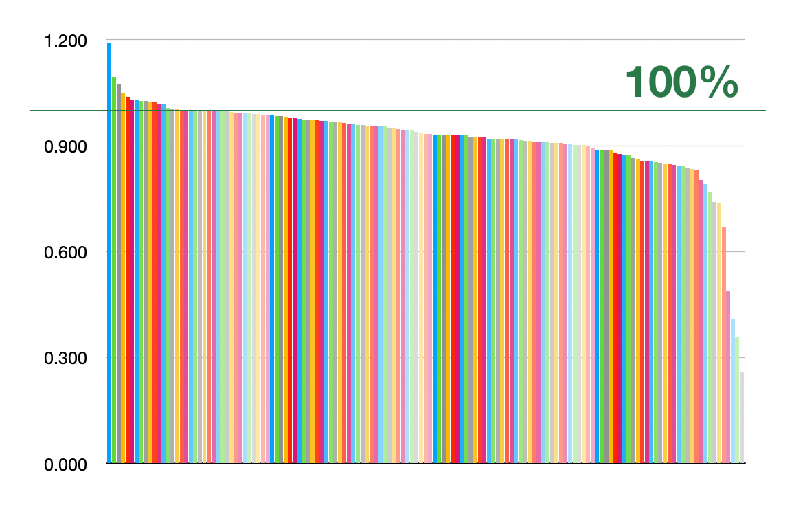
Running the benchmark suite – 13% faster:
! Zig VM
IN: scratchpad gc [ timing-benchmarks ] time
Running time: 438.671019723 seconds

! C++ VM
IN: scratchpad gc [ timing-benchmarks ] time
Running time: 508.235989841 seconds
And you can see that if we sort the benchmarks by percent improvements (worse
to better), some benchmarks that are bignum heavy are much faster, some
are a little faster, and a few have regressed:
Comparing lines of code – 67% more – with fewer files:
# Zig VM
━━━━━━━━━━━━━━━━━━━━━━━━━━━━━━━━━━━━━━━━━━━━━━━━━━━━━━━━━━━━━━━━━━━━━━━━━━━━━━━━━
 Language              Files        Lines         Code     Comments       Blanks
━━━━━━━━━━━━━━━━━━━━━━━━━━━━━━━━━━━━━━━━━━━━━━━━━━━━━━━━━━━━━━━━━━━━━━━━━━━━━━━━━
 Zig                      51        29034        21032         3761         4241
━━━━━━━━━━━━━━━━━━━━━━━━━━━━━━━━━━━━━━━━━━━━━━━━━━━━━━━━━━━━━━━━━━━━━━━━━━━━━━━━━
 Total                    51        29034        21032         3761         4241
━━━━━━━━━━━━━━━━━━━━━━━━━━━━━━━━━━━━━━━━━━━━━━━━━━━━━━━━━━━━━━━━━━━━━━━━━━━━━━━━━

# C++ VM
━━━━━━━━━━━━━━━━━━━━━━━━━━━━━━━━━━━━━━━━━━━━━━━━━━━━━━━━━━━━━━━━━━━━━━━━━━━━━━━━━
 Language              Files        Lines         Code     Comments       Blanks
━━━━━━━━━━━━━━━━━━━━━━━━━━━━━━━━━━━━━━━━━━━━━━━━━━━━━━━━━━━━━━━━━━━━━━━━━━━━━━━━━
 Assembly                  1            5            5            0            0
 GNU Style Assembly        3          205          150           20           35
 C                         1          408          323            2           83
 C Header                  1          270          220            2           48
 C++                      58         9911         7597          777         1537
 C++ Header               84         5967         4297          606         1064
━━━━━━━━━━━━━━━━━━━━━━━━━━━━━━━━━━━━━━━━━━━━━━━━━━━━━━━━━━━━━━━━━━━━━━━━━━━━━━━━━
 Total                   148        16776        12592         1407         2767
━━━━━━━━━━━━━━━━━━━━━━━━━━━━━━━━━━━━━━━━━━━━━━━━━━━━━━━━━━━━━━━━━━━━━━━━━━━━━━━━━
Comparing binary sizes – 77% larger:
# Zig VM
-rwxrwxr-x 1 user  staff   758K Mar 17 11:25 factor

# C++ VM
-rwxrwxr-x 1 user  staff   430K Mar  8 13:39 factor
Next Steps
So, where does this go from here?
Well, besides making it also work on Windows, launch graphical programs properly, support compressed images, maybe support 32-bit, generally ensuring that it is a fully bug-free re-implementation of Factor, and investigating why the binaries are larger.
Perhaps it is an opportunity to re-think how the Factor bootstrap process works, to reduce the amount of functions a Factor VM should support, to run Factor in WASM with an optimizing compiler, to implement a simple Factor interpreter, or challenge our assumptions on what it means to be a Factor.
Or, it could just be a fun experiment using Zig. Let’s see!
John Benediktsson: Standard Deviation
Standard deviation is “a measure of the amount of variation of the values of a variable about its mean.”. It’s a useful measure from statistics, and std in the math.statistics vocabulary included with Factor.
I bumped into this – um, are they still called tweets? – today:
Word with the lowest standard deviation of letter position in the alphabet, for each length pic.twitter.com/caHYDDpyBx
— Adam Aaronson (@aaaronson) February 4, 2026
Of course, I wondered how that looks for the /usr/share/dict/words on my computer:
IN: scratchpad "/usr/share/dict/words" utf8 file-lines
               [ length ] collect-by
               [ [ std ] minimum-by ] assoc-map
               sort-keys values
               [ dup std "%s: %s\n" printf ] each
A: 0.0
aa: 0.0
aba: 0.5773502691896257
baba: 0.5773502691896257
abaca: 0.8944271909999159
bacaba: 0.816496580927726
deedeed: 0.5345224838248488
poroporo: 1.3093073414159542
susurrous: 1.9364916731037085
beefheaded: 1.9578900207451218
cabbagehead: 2.46429041972071
fiddledeedee: 2.424621182533032
promonopolist: 2.911075226502911
monogonoporous: 3.1830595551871363
prophototropism: 3.5023801430836525
philophilosophos: 3.855731664245668
sulphophosphorous: 4.227013964824759
chemicoengineering: 4.556472090169843
plutonometamorphism: 5.220293285659733
encephalomeningocele: 4.871776937249466
philosophicoreligious: 5.014740177478695
philosophicohistorical: 5.485320828241917
philosophicotheological: 5.2090678006509625
scientificophilosophical: 5.538894097749744
antidisestablishmentarianism: 6.7081053397123425
Interesting, both similar and different. Well, it’s pretty close and also pretty obvious we are using slightly different dictionaries. I’m not sure what deedeed or poroporo mean and they aren’t in the SCRABBLE Players Dictionary.
Anyway, fun!
John Benediktsson: PBRT
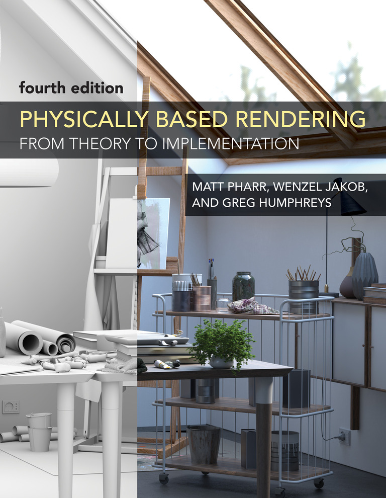
PBRT is an impressive photorealistic rendering system:
From movies to video games, computer-rendered images are pervasive today. Physically Based Rendering introduces the concepts and theory of photorealistic rendering hand in hand with the source code for a sophisticated renderer.
The fourth edition of their book is now available on Amazon as well as freely available online.
I thought it would be fun to explore the PBRT v4 file format using Factor.
Here’s a short example pbrt file from their website:
LookAt 3 4 1.5  # eye
       .5 .5 0  # look at point
       0 0 1    # up vector
Camera "perspective" "float fov" 45

Sampler "halton" "integer pixelsamples" 128
Integrator "volpath"
Film "rgb" "string filename" "simple.png"
     "integer xresolution" [400] "integer yresolution" [400]

WorldBegin

# uniform blue-ish illumination from all directions
LightSource "infinite" "rgb L" [ .4 .45 .5 ]

# approximate the sun
LightSource "distant"  "point3 from" [ -30 40  100 ]
   "blackbody L" 3000 "float scale" 1.5

AttributeBegin
  Material "dielectric"
  Shape "sphere" "float radius" 1
AttributeEnd

AttributeBegin
  Texture "checks" "spectrum" "checkerboard"
          "float uscale" [16] "float vscale" [16]
          "rgb tex1" [.1 .1 .1] "rgb tex2" [.8 .8 .8]
  Material "diffuse" "texture reflectance" "checks"
  Translate 0 0 -1
  Shape "bilinearmesh"
      "point3 P" [ -20 -20 0   20 -20 0   -20 20 0   20 20 0 ]
      "point2 uv" [ 0 0   1 0    1 1   0 1 ]
AttributeEnd
And this is what it might look like:
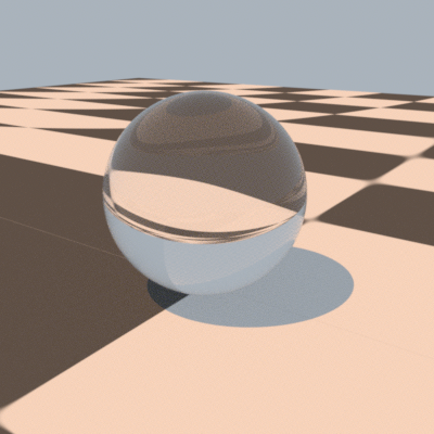
Using our new pbrt vocabulary, we can convert that text into a set of tuples that we could do computations on, or potentially look into rendering or processing. And, of course, it also supports round-tripping back and forth from text to tuples.
{
    T{ pbrt-look-at
        { eye-x 3 }
        { eye-y 4 }
        { eye-z 1.5 }
        { look-x 0.5 }
        { look-y 0.5 }
        { look-z 0 }
        { up-x 0 }
        { up-y 0 }
        { up-z 1 }
    }
    T{ pbrt-camera
        { type "perspective" }
        { params
            {
                T{ pbrt-param
                    { type "float" }
                    { name "fov" }
                    { values { 45 } }
                }
            }
        }
    }
    T{ pbrt-sampler
        { type "halton" }
        { params
            {
                T{ pbrt-param
                    { type "integer" }
                    { name "pixelsamples" }
                    { values { 128 } }
                }
            }
        }
    }
    T{ pbrt-integrator { type "volpath" } { params { } } }
    T{ pbrt-film
        { type "rgb" }
        { params
            {
                T{ pbrt-param
                    { type "string" }
                    { name "filename" }
                    { values { "simple.png" } }
                }
                T{ pbrt-param
                    { type "integer" }
                    { name "xresolution" }
                    { values { 400 } }
                }
                T{ pbrt-param
                    { type "integer" }
                    { name "yresolution" }
                    { values { 400 } }
                }
            }
        }
    }
    T{ pbrt-world-begin }
    T{ pbrt-light-source
        { type "infinite" }
        { params
            {
                T{ pbrt-param
                    { type "rgb" }
                    { name "L" }
                    { values { 0.4 0.45 0.5 } }
                }
            }
        }
    }
    T{ pbrt-light-source
        { type "distant" }
        { params
            {
                T{ pbrt-param
                    { type "point3" }
                    { name "from" }
                    { values { -30 40 100 } }
                }
                T{ pbrt-param
                    { type "blackbody" }
                    { name "L" }
                    { values { 3000 } }
                }
                T{ pbrt-param
                    { type "float" }
                    { name "scale" }
                    { values { 1.5 } }
                }
            }
        }
    }
    T{ pbrt-attribute-begin }
    T{ pbrt-material { type "dielectric" } { params { } } }
    T{ pbrt-shape
        { type "sphere" }
        { params
            {
                T{ pbrt-param
                    { type "float" }
                    { name "radius" }
                    { values { 1 } }
                }
            }
        }
    }
    T{ pbrt-attribute-end }
    T{ pbrt-attribute-begin }
    T{ pbrt-texture
        { name "checks" }
        { value-type "spectrum" }
        { class "checkerboard" }
        { params
            {
                T{ pbrt-param
                    { type "float" }
                    { name "uscale" }
                    { values { 16 } }
                }
                T{ pbrt-param
                    { type "float" }
                    { name "vscale" }
                    { values { 16 } }
                }
                T{ pbrt-param
                    { type "rgb" }
                    { name "tex1" }
                    { values { 0.1 0.1 0.1 } }
                }
                T{ pbrt-param
                    { type "rgb" }
                    { name "tex2" }
                    { values { 0.8 0.8 0.8 } }
                }
            }
        }
    }
    T{ pbrt-material
        { type "diffuse" }
        { params
            {
                T{ pbrt-param
                    { type "texture" }
                    { name "reflectance" }
                    { values { "checks" } }
                }
            }
        }
    }
    T{ pbrt-translate { x 0 } { y 0 } { z -1 } }
    T{ pbrt-shape
        { type "bilinearmesh" }
        { params
            {
                T{ pbrt-param
                    { type "point3" }
                    { name "P" }
                    { values
                        { -20 -20 0 20 -20 0 -20 20 0 20 20 0 }
                    }
                }
                T{ pbrt-param
                    { type "point2" }
                    { name "uv" }
                    { values { 0 0 1 0 1 1 0 1 } }
                }
            }
        }
    }
    T{ pbrt-attribute-end }
}
This is available now in the development version of Factor!
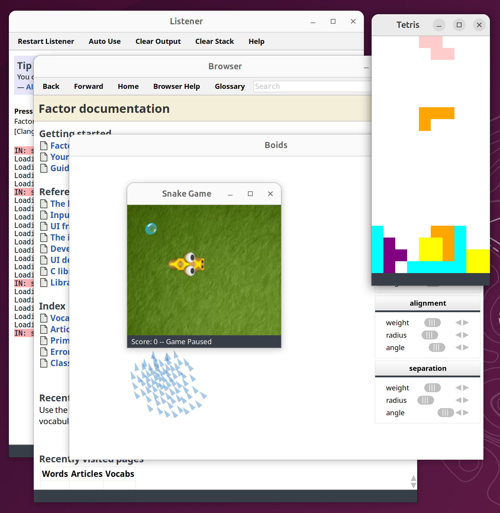
John Benediktsson: Migrating to GTK3
Factor has a native ui-backend that allows us to render our UI framework using OpenGL on top of platform-specific APIs for our primary targets of Linux, macOS, and Windows.
On Linux, for a long time that has meant using the
GTK2 library, which has also meant using
X11 and an old library
called libgtkglext which provides a way to use OpenGL within GTK
windows. Well, Linux has moved on and is now pushing
Wayland as the “replacement for the X11
window system protocol and architecture with the aim to be easier to
develop, extend, and maintain”. Most modern Linux distributions have moved
to GTK3 or GTK4 and abstraction libraries like
libepoxy for working with OpenGL and
others for supporting both X11 and Wayland renderers.
I was reminded of this after our recent Factor 0.101 release when someone asked the question:
Does that message mean that Factor still relies on GTK2? IIRC it was EOL:ed around 2020.
Well, this is embarassing – yeah it sure does! Or rather – yes it sure did.
I got motivated to look into what it would take to support GTK3 or GTK4. We had a pull request that was working through adding support for GTK4. After merging that, and modifying it to also provide GTK3 support, I re-discovered that our OpenGL rendering was generally using OpenGL 1.x pipelines and that would not work in a GTK3+ world.
So, after adding OpenGL 3.x support for most of the things our user interface needs, and migrating from GTK 2.x to GTK3, we now have experimental nightly builds using the GTK3 backend:
You can revert to the older GTK2 backend by applying this diff and then performing a fresh bootstrap:
diff --git a/basis/bootstrap/ui/ui.factor b/basis/bootstrap/ui/ui.factor
index 2974e530f9..416704ce29 100644
--- a/basis/bootstrap/ui/ui.factor
+++ b/basis/bootstrap/ui/ui.factor
@@ -12,6 +12,6 @@ IN: bootstrap.ui
     {
         { [ os macos? ] [ "ui.backend.cocoa" ] }
         { [ os windows? ] [ "ui.backend.windows" ] }
-        { [ os unix? ] [ "ui.backend.gtk3" ] }
+        { [ os unix? ] [ "ui.backend.gtk2" ] }
     } cond
 ] if* require
diff --git a/basis/opengl/gl/extensions/extensions.factor b/basis/opengl/gl/extensions/extensions.factor
index 2d408e93bb..51394eeb4a 100644
--- a/basis/opengl/gl/extensions/extensions.factor
+++ b/basis/opengl/gl/extensions/extensions.factor
@@ -7,7 +7,7 @@ ERROR: unknown-gl-platform ;
 << {
     { [ os windows? ] [ "opengl.gl.windows" ] }
     { [ os macos? ]  [ "opengl.gl.macos" ] }
-    { [ os unix? ] [ "opengl.gl.gtk3" ] }
+    { [ os unix? ] [ "opengl.gl.gtk2" ] }
     [ unknown-gl-platform ]
 } cond use-vocab >>
It seems like the newer OpenGL 3.x functions might introduce some lag which is visible when scrolling on some installations, perhaps by not caching certain things that were cached in the OpenGL 1.x code paths. There will need to be some improvements before we are ready to release it, but it is plenty usable as-is.
I also migrated our macOS backend to use the OpenGL 3.x functions as well to allow us to more broadly test and improve these new rendering paths.
This is available in the latest development version.
John Benediktsson: DNS LOC Records
DNS is the Domain Name System and is the backbone of the internet:
Most prominently, it translates readily memorized domain names to the numerical IP addresses needed for locating and identifying computer services and devices with the underlying network protocols. The Domain Name System has been an essential component of the functionality of the Internet since 1985.
It is also an oft-cited reason for service outages, with a funny decade-old r/sysadmin meme:

Factor has a DNS vocabulary that supports querying and parsing responses from nameservers:
IN: scratchpad USE: tools.dns

IN: scratchpad "google.com" host
google.com has address 142.250.142.113
google.com has address 142.250.142.138
google.com has address 142.250.142.100
google.com has address 142.250.142.101
google.com has address 142.250.142.102
google.com has address 142.250.142.139
google.com has IPv6 address 2607:f8b0:4023:1c01:0:0:0:8b
google.com has IPv6 address 2607:f8b0:4023:1c01:0:0:0:8a
google.com has IPv6 address 2607:f8b0:4023:1c01:0:0:0:64
google.com has IPv6 address 2607:f8b0:4023:1c01:0:0:0:65
google.com mail is handled by 10 smtp.google.com
Recently, I bumped into an old post on the Cloudflare
blog about The weird and wonderful world of
DNS LOC
records
and realized that we did not properly support parsing RFC
1876 which specifies a format
for returning LOC or location record specifying the physical
location of a service.
At the time of the post, Cloudflare indicated they handle “millions of DNS records; of those just 743 are LOCs.”. I found a webpage that lists sites supporting DNS LOC and contains only nine examples.
It is not widely used, but it is very cool.
You can use the dig command
to query for a LOC record and see what is returned:
$ dig alink.net LOC
alink.net.              66      IN      LOC     37 22 26.000 N 122 1 47.000 W 30.00m 30m 30m 10m
The fields that were returned include:
- latitude (37° 22’ 26.00" N)
- longitude (122° 1’ 47.00" W)
- altitude (30.00m)
- horizontal precision (30m)
- vertical precision (30m)
- entity size estimate (10m)
In Factor 0.101, the field is available and returned as bytes but not parsed:
IN: scratchpad "alink.net" dns-LOC-query answer-section>> ...
{
    T{ rr
        { name "alink.net" }
        { type LOC }
        { class IN }
        { ttl 300 }
        { rdata
            B{
                0 51 51 19 136 5 2 80 101 208 181 8 0 152 162 56
            }
        }
    }
}
Of course, I love odd uses of technology like Wikipedia over
DNS and I thought
Factor should probably add proper support for the
LOC record!
First, we define a tuple
class to hold the
LOC record fields:
TUPLE: loc size horizontal vertical lat lon alt ;
Next, we parse the LOC record, converting sizes (in centimeters),
lat/lon (in degrees), and altitude (in centimeters):
: parse-loc ( -- loc )
    loc new
        read1 0 assert=
        read1 [ -4 shift ] [ 4 bits ] bi 10^ * >>size
        read1 [ -4 shift ] [ 4 bits ] bi 10^ * >>horizontal
        read1 [ -4 shift ] [ 4 bits ] bi 10^ * >>vertical
        4 read be> 31 2^ - 3600000 / >>lat
        4 read be> 31 2^ - 3600000 / >>lon
        4 read be> 10000000 - >>alt ;
We hookup the LOC type to be parsed properly:
M: LOC parse-rdata 2drop parse-loc ;
And then build a word to print the location nicely:
: LOC. ( name -- )
    dns-LOC-query answer-section>> [
        rdata>> {
            [ lat>> [ abs 1 /mod 60 * 1 /mod 60 * ] [ neg? "S" "N" ? ] bi ]
            [ lon>> [ abs 1 /mod 60 * 1 /mod 60 * ] [ neg? "W" "E" ? ] bi ]
            [ alt>> 100 / ]
            [ size>> 100 /i ]
            [ horizontal>> 100 /i ]
            [ vertical>> 100 /i ]
        } cleave "%d %d %.3f %s %d %d %.3f %s %.2fm %dm %dm %dm\n" printf
    ] each ;
And, finally, we can give it a try!
IN: scratchpad "alink.net" LOC.
37 22 26.000 N 122 1 47.000 W 30.00m 30m 30m 10m
Yay, it matches!
This is available in the latest development version.
John Benediktsson: Factor 0.101 now available
“Keep thy airspeed up, lest the earth come from below and smite thee.” - William Kershner
I’m very pleased to announce the release of Factor 0.101!
| OS/CPU | Windows | Mac OS | Linux |
|---|---|---|---|
| x86 | 0.101 | 0.101 | |
| x86-64 | 0.101 | 0.101 | 0.101 |
Source code: 0.101
This release is brought to you with almost 700 commits by the following individuals:
Aleksander Sabak, Andy Kluger, Cat Stevens, Dmitry Matveyev, Doug Coleman, Giftpflanze, John Benediktsson, Jon Harper, Jonas Bernouli, Leo Mehraban, Mike Stevenson, Nicholas Chandoke, Niklas Larsson, Rebecca Kelly, Samuel Tardieu, Stefan Schmiedl, @Bruno-366, @bobisageek, @coltsingleactionarmyocelot, @inivekin, @knottio, @timor
Besides some bug fixes and library improvements, I want to highlight the following changes:
- Moved the UI to render buttons and scrollbars rather than using images, which allows easier theming.
- Fixed HiDPI scaling on Linux and Windows, although it currently doesn’t update the window settings when switching between screens with different scaling factors.
- Update to Unicode 17.0.0.
- Plugin support for the Neovim editor.
Some possible backwards compatibility issues:
- The argument order to
ltakewas swapped to be more consistent with words likehead. - The
environmentvocabulary on Windows now supports disambiguatingfand""(empty) values - The
misc/atomfolder was removed in favor of the factor/atom-language-factor repo. - The
misc/Factor.tmbundlefolder was removed in favor of the factor/factor.tmbundle repo. - The
misc/vimfolder was removed in favor of the factor/factor.vim repo. - The
httpvocabularyrequesttuple had a slot rename frompost-datatodata. - The
furnace.asidesvocabulary had a slot rename frompost-datatodata, and might require runningALTER TABLE asides RENAME COLUMN "post-data" TO data;. - The
html.streamsvocabulary was renamed toio.streams.html - The
pdf.streamsvocabulary was renamed toio.streams.pdf
What is Factor
Factor is a concatenative, stack-based programming language with high-level features including dynamic types, extensible syntax, macros, and garbage collection. On a practical side, Factor has a full-featured library, supports many different platforms, and has been extensively documented.
The implementation is fully compiled for performance, while still supporting interactive development. Factor applications are portable between all common platforms. Factor can deploy stand-alone applications on all platforms. Full source code for the Factor project is available under a BSD license.
New libraries:
- base92: adding support for Base92 encoding/decoding
- bitcask: implementing the Bitcask key/value database
- bluesky: adding support for the BlueSky protocol
- calendar.holidays.world: adding some new holidays including World Emoji Day
- classes.enumeration: adding enumeration classes and new
ENUMERATION:syntax word - colors.oklab: adding support for OKLAB color space
- colors.oklch: adding support for OKLCH color space
- colors.wavelength: adding
wavelength>rgba - combinators.syntax: adding experimental combinator syntax words
@[,*[, and&[, and short-circuitingn&&[,n||[,&&[and||[ - continuations.extras: adding
with-datastacksanddatastack-states - dotenv: implementing support for Dotenv files
- edn: implementing support for Extensible Data Notation
- editors.cursor: adding support for the Cursor editor
- editors.rider: adding support for the JetBrains Rider editor
- gitignore: parser for
.gitignorefiles - http.json: promoted
json.httpand added some useful words - io.streams.farkup: a Farkup formatted stream protocol
- io.streams.markdowns: a Markdown formatted stream protocol
- locals.lazy: prototype of emit syntax
- monadics: alternative vocabulary for using Haskell-style monads, applicatives, and functors
- multibase: implementation of Multibase
- pickle: support for the Pickle serialization format
- persistent.hashtables.identity: support an identity-hashcode version of persisent hashtables
- raylib.live-coding: demo of a vocabulary to do “live coding” of Raylib programs
- rdap: support for the Registration Data Access Protocol
- reverse: implementation of the std::flip
- slides.cli: simple text-based command-line interface for slides
- tools.highlight: command-line syntax-highlighting tool
- tools.random: command-line random generator tool
- ui.pens.rounded: adding rounded corner pen
- ui.pens.theme: experimental themed pen
- ui.tools.theme: some words for updating UI developer tools themes
Improved libraries:
- alien.syntax: added
C-LIBRARY:syntax word - assocs.extras: added
nzipandnunzip,map-zipandmap-unzipmacros - base32: adding the human-oriented Base32 encoding via
zbase32>and>zbase32 - base64: minor performance improvement
- benchmark: adding more benchmarks
- bootstrap.assembler: fixes for ARM-64
- brainfuck: added
BRAINFUCK:syntax word andinterpret-brainfuck - bson: use linked-assocs to preserve order
- cache: implement
M\ cache-assoc delete-at - calendar: adding
year<,year<=,year>,year>=words - calendar.format: parse human-readable and elapsed-time output back into duration objects
- cbor: use linked-assocs to preserve order
- classes.mixin: added
definerimplementation - classes.singleton: added
definerimplementation - classes.tuple: added
tuple>slots, renametuple>arraytopack-tupleand>tupletounpack-tuple. - classes.union: added
definerimplementation - checksums.sha: some 20-40% performance improvements
- command-line: allow passing script name of
-to use stdin - command-line.parser: support for Argument Parser Commands
- command-line.startup: document
-qquiet mode flag - concurrency.combinators: faster
parallel-mapandparallel-assoc-mapusing a count-down latch - concurrency.promises: 5-7% performance improvement
- continuations: improve docs and fix stack effect for
ifcc - countries: adding
CQcountry code for Sark - cpu.architecture: fix
*-branchstack effects - cpu.arm: fixes for ARM-64
- crontab: added
parse-crontabwhich ignores blank lines and comments - db: making
query-eachrow-polymorphic - delegate.protocols: adding
keysandvaluestoassoc-protocol - discord: better support for network disconnects, added a configurable retry interval
- discord.chatgpt-bot: some fixes for LM Studio
- editors: make the editor restart nicer looking
- editors.focus: support open-file-to-line-number on newer releases, support Linux and Window
- editors.zed: support use of Zed on Linux
- endian: faster endian conversions of c-ptr-like objects
- environment: adding
os-env? - eval: move datastack and error messages to stderr
- fonts: make
<font>take a name, easier defaults - furnace.asides: rename
post-dataslot onasidetuples todata - generalizations: moved some dip words to shuffle
- help.tour: fix some typos/grammar
- html.templates.chloe: improve use of
CDATAtags for unescaping output - http: rename
post-dataslot onrequesttuples todata - http.json: adding
http-jsonthat doesn’t return the response object - http.websockets: making
read-websocket-looprow-polymorphic - ini-file: adding
ini>file,file>ini, and useLH{ }to preserve configuration order - io.encodings.detect: adding
utf7detection - io.encodings.utf8: adding
utf8-bomto handle optional BOM - io.random: speed up
random-lineandrandom-lines - io.streams.ansi: adding documentation and tests, support dim foreground on terminals that support it
- io.streams.escape-codes: adding documentation and tests
- ip-parser: adding IPV4 and IPV6 network words
- kernel: adding
until*, fix docs forand*andor* - linked-sets: adding
LS{syntax word - lists.lazy: changed the argument order in
ltake - macho: support a few more link edit commands
- make: adding
,%for apush-atvariant - mason.release.tidy: cleanup a few more git artifacts
- math.combinatorics: adding counting words
- math.distances: adding
jaro-distanceandjaro-winkler-distance - math.extras: added
all-removals, support Recamán’s sequence, and Tribonacci Numbers - math.factorials: added
subfactorial - math.functions: added “closest to zero” modulus
- math.parser: improve ratio parsing for consistency
- math.primes: make
prime?safe from non-integer inputs - math.runge-kutta: make generalized improvements to the Runge-Kutta solver
- math.similarity: adding
jaro-similarity,jaro-winkler-similarity, andtrigram-similarity - math.text.english: fix issue with very large and very small floats
- metar: updated the abbreviations glossary
- mime.types: updating
mime.typesfile - msgpack: use linked-assocs to preserve order
- qw: adding
qw:syntax - path-finding: added
find-path* - peg.parsers: faster
list-ofandlist-of-many - progress-bars.models: added
with-progress-display,map-with-progress-bar,each-with-progress-bar, andreduce-with-progress-bar - raylib: adding
trace-logandset-trace-log-level, updated to Raylib 5.5 - readline-listener: store history across sessions, support color on terminals that support it
- robohash: support for
"set4","set5", and"set6"types - sequences: rename
midpoint@tomidpoint, fastereach-fromandmap-reduceon slices - sequences.extras: adding
find-nth,find-nth-last,subseq-indices,deep-nth,deep-nth-of,2none?,filter-errors,reject-errors,all-same?,adjacent-differences, andpartial-sum. - sequences.generalizations: fix
?firstnand?lastnfor string inputs, removed(nsequence)which duplicatesset-firstn-unsafe - sequences.prefixed: swap order of
<prefixed>arguments to matchprefix - sequences.repeating: adding
<cycles-from>andcycle-from - sequences.snipped: fixed out-of-bounds issues
- scryfall: update for duskmourn
- shuffle: improve stack-checking of
shuffle(syntax, addedSHUFFLE:syntax,nreverse - sorting: fix
sort-withto apply the quot with access to the stack below - sorting.human: implement human sorting improved
- system-info.macos: adding “Tahoe” code-name for macOS 26
- terminfo: add words for querying specific output capabilities
- threads: define a generalized
linked-threadwhich used to be forconcurrency.mailboxesonly - toml: use linked-assocs to preserve order, adding
>tomlandwrite-toml - tools.annotations: adding
<WATCH ... WATCH>syntax - tools.deploy: adding a command-line interface for deploy options
- tools.deploy.backend: fix boot image location in system-wide installations
- tools.deploy.unix: change binary name to append
.outto fix conflict with vocab resources - tools.directory-to-file: better test file metrics, print filename for editing
- tools.memory: adding
heap-stats-ofarbitrary sequence of instances, andtotal-sizesize of everything pointed to by an object - txon: use linked-assocs to preserve order
- ui: adding
adjust-font-size - ui.gadgets.buttons: stop using images and respect theme colors
- ui.gadgets.sliders: stop using images and respect theme colors
- ui.theme.base16: adding a lot more (270!) Base16 Themes
- ui.tools: adding font-sizing keyboard shortcuts
- ui.tools.browser: more responsive font sizing
- ui.tools.listener: more responsive font sizing, adding some UI listener styling
- ui.tools.listener.completion: allow spaces in history search popup
- unicode: update to Unicode 17.0.0
- webapps.planet: improve CSS for
videotags - words: adding
define-temp-syntax - zoneinfo: update to version 2025b
Removed libraries
ui.theme.images
VM Improvements:
- More work on ARM64 backend (fix set-callstack, fix generic dispatch)
Blogroll
- Chris Double
- Daniel Ehrenberg
- Doug Coleman
- Jeremy Hughes
- Joe Groff
- John Benediktsson
- Phil Dawes
- Samuel Tardieu
- Slava Pestov
planet-factor is an Atom/RSS aggregator that collects the contents of Factor-related blogs. It is inspired by Planet Lisp.